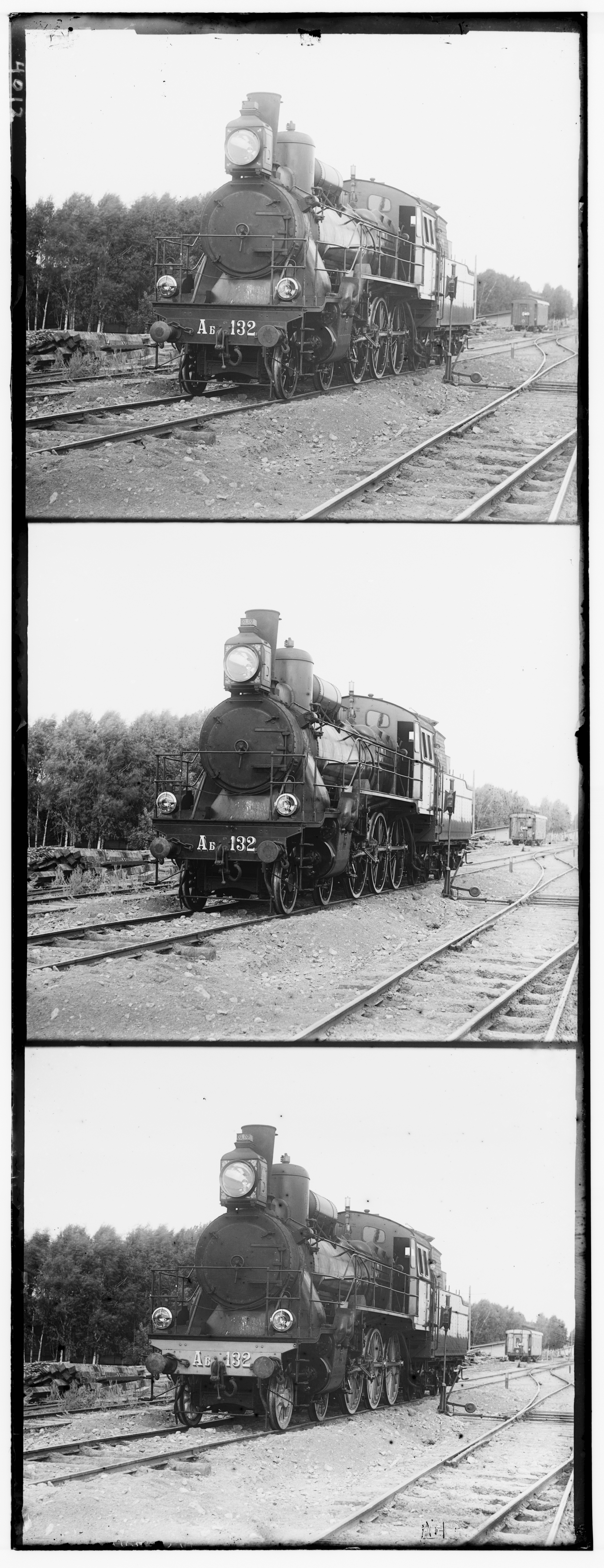
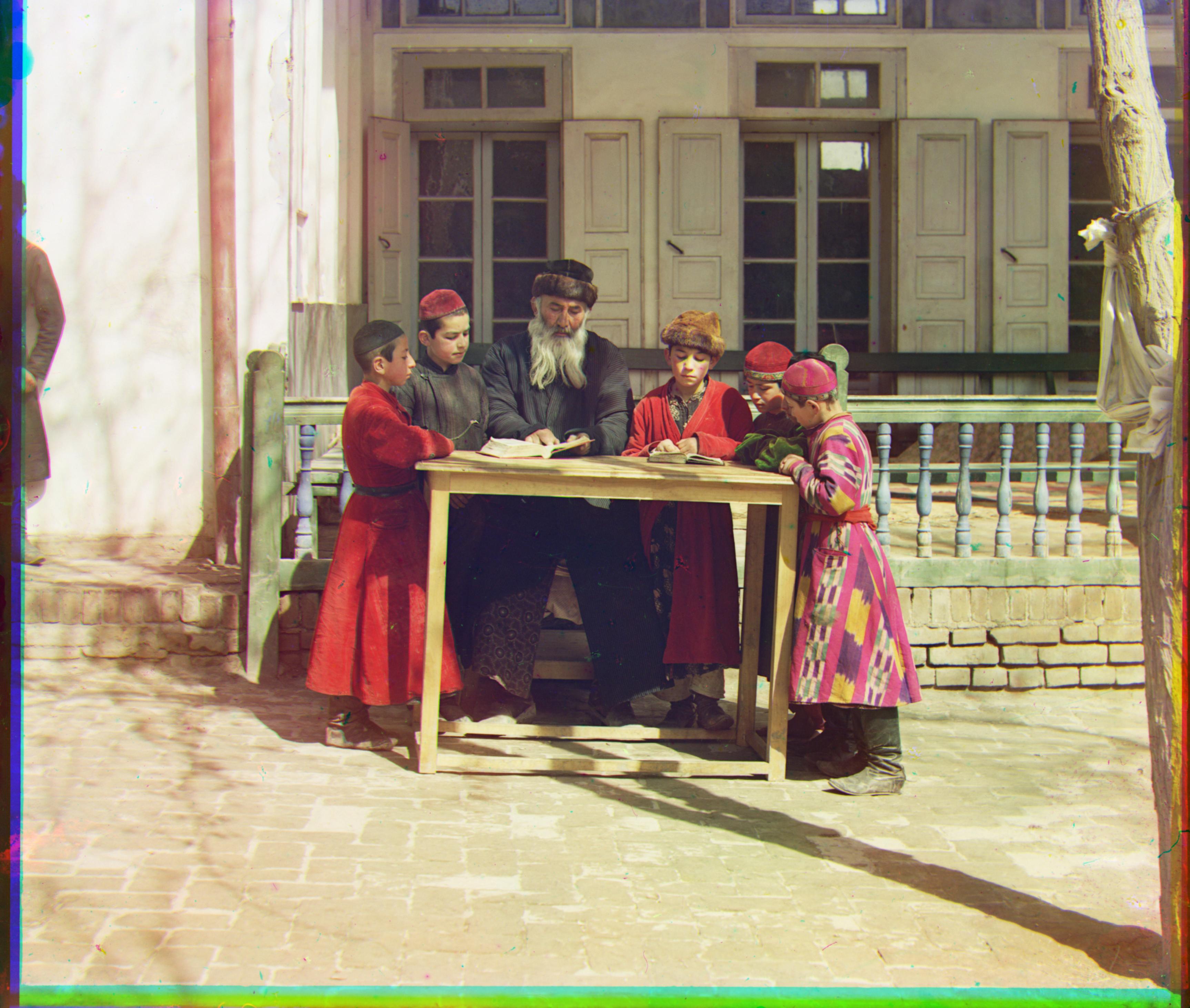
Figure 1. Original plate (00458u)
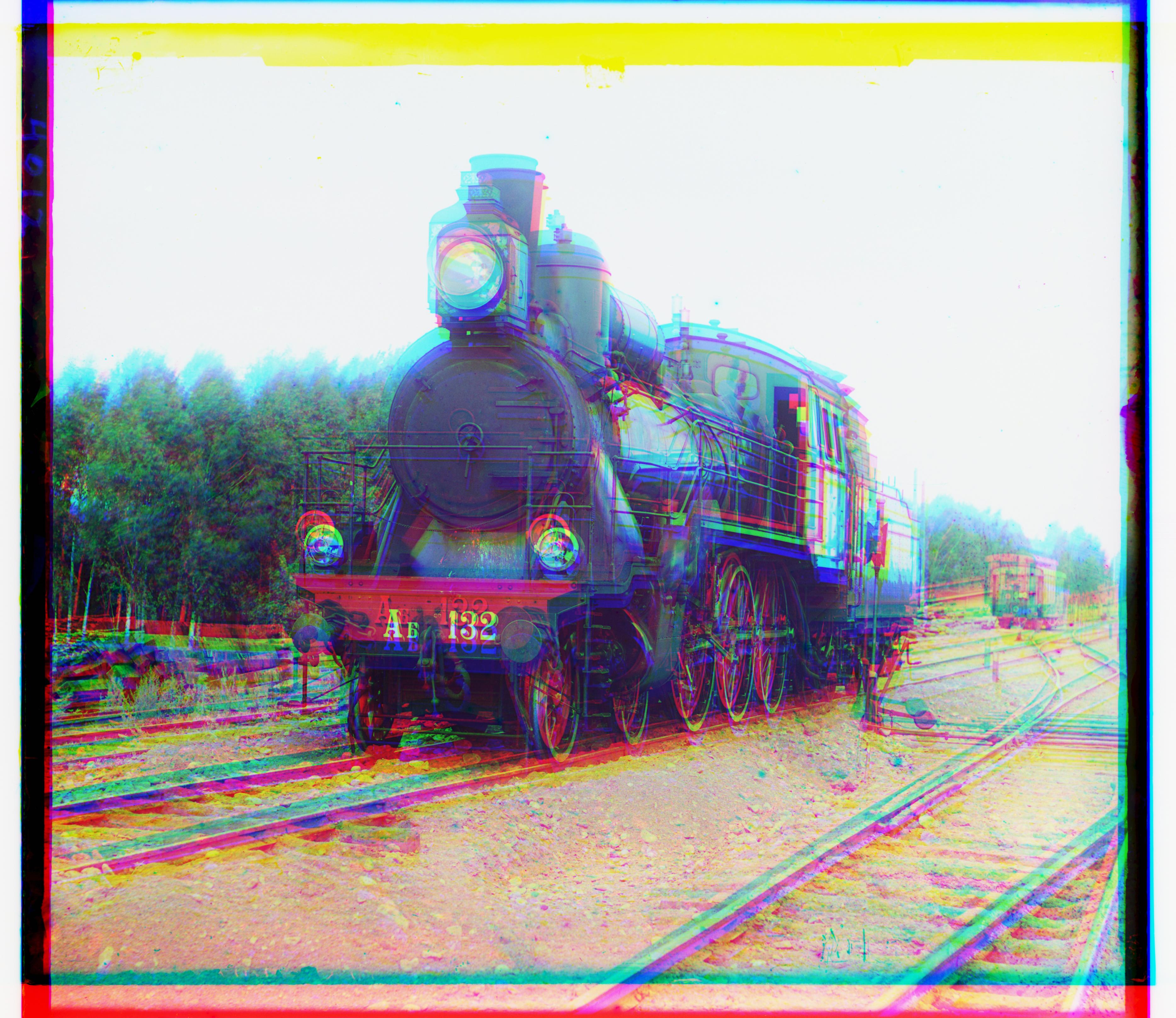
Figure 2. Naive B/G/R stack, zero shift
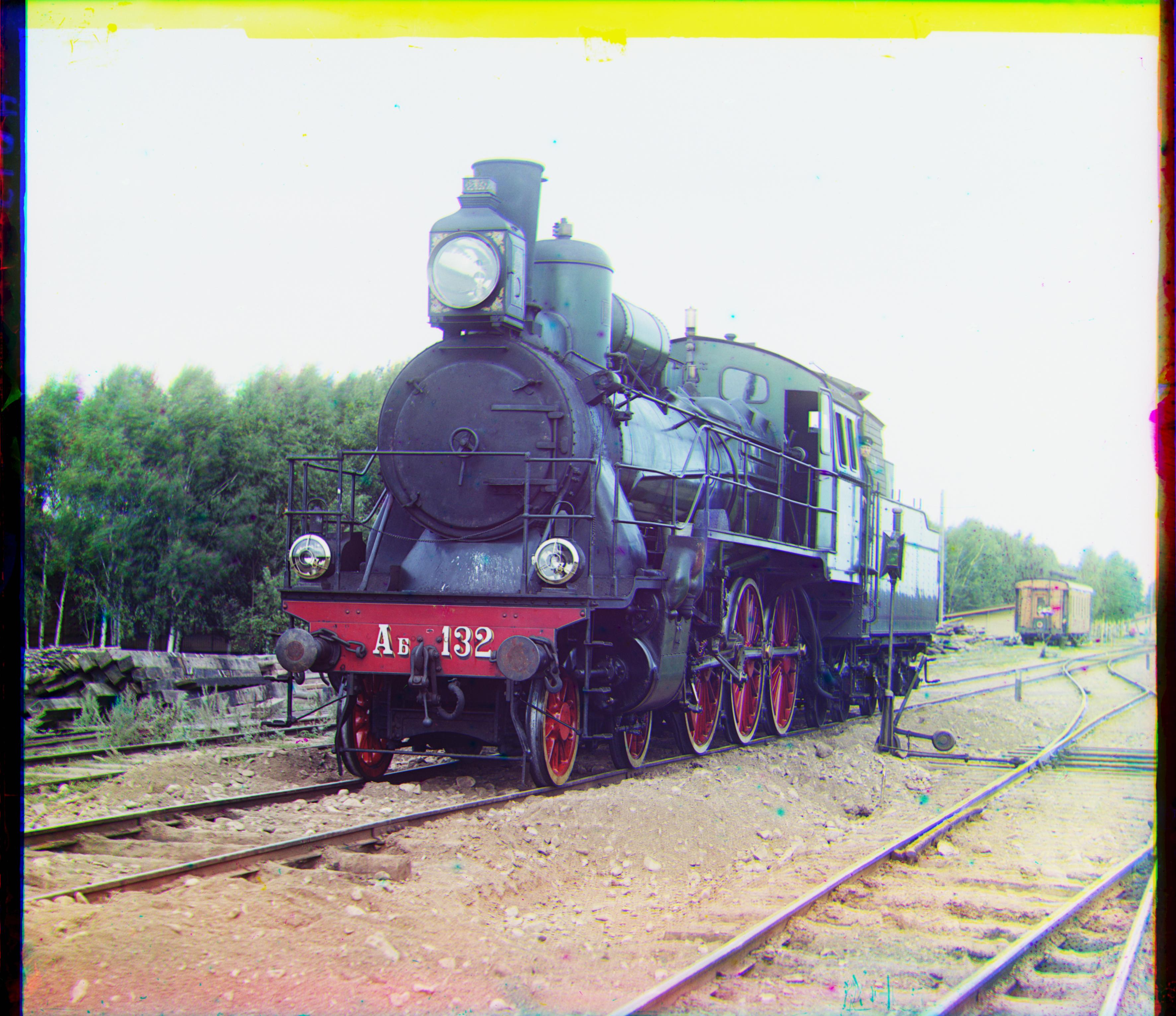
Figure 3. After alignment: G (9, 15), R (15, 15)
SYDE 671, Assignment 1 — Muhammad Farooq Memon
Around 1907 Sergei Prokudin-Gorskii shot the same scene three times through blue, green and red filters onto one glass plate. Stack the three exposures as R, G, B and you get a color photo. The digitized plates come as one grayscale image with the exposures stacked vertically: blue on top, green in the middle, red at the bottom.
The catch is that the exposures aren't lined up, so the job is finding how far to shift G and R so they land on B. Sign convention, used everywhere in my code (I got burned once by flipping it):
+dx = right -dx = left +dy = down -dy = upFigure 1. Original plate (00458u)
Figure 2. Naive B/G/R stack, zero shift
Figure 3. After alignment: G (9, 15), R (15, 15)
From glass plate to color photograph. Simply stacking the three exposures gives colored fringes and ghosted edges; alignment removes the displacement between them.
The color information is already in the three channels. The only problem is that they're spatially displaced, and that's what the rest of this page is about.
For each candidate shift (dx, dy) I compare G (or R) against B and keep the best score. I only score a fixed 12% interior crop, because the plate borders and scan junk otherwise pull the best match toward the borders instead of the photo.
L2 measures pixel-by-pixel squared differences, where a lower score means a better alignment. The naive way to compute this across a search window is to create a temporary difference image (A - B) for every shift, square every pixel, and sum them up. For a typical 31 x 31 search window, that means allocating and processing 961 temporary images in memory, which is unnecessarily slow.
Instead, I expand the formula algebraically:
||A - B||² = ||A||² + ||B||² - 2(A · B)
Because the reference slice A never changes during the search, its squared sum ||A||² is identical for all 961 candidates. I calculate ||A||² once before entering the search loop and reuse it. During the search, the code only needs to compute the dot product A · B and the target energy ||B||² per candidate. This avoids creating temporary difference arrays entirely and speeds up the search loop significantly.
NCC treats the image regions as vectors and measures their alignment angle using dot products normalized by vector lengths: (A · B) / (||A|| · ||B||). Higher scores mean better alignment, topping out at 1.0 for a perfect match.
In theory (in my case I didn't see much difference XD), NCC is much better suited for RGB glass plate alignment than L2 because raw pixel values vary naturally between color filters, for example, a bright blue garment appears light in the blue channel but dark in the red channel. Standard L2 penalizes these natural intensity gaps heavily, whereas NCC normalizes by brightness magnitude so it focuses on structural patterns instead of absolute lighting.
Similar to L2, NCC is optimized by precomputing the reference norm ||A|| outside the candidate loop, leaving only the dot product A · B and candidate norm ||B|| to be computed per shift.
Here are some images created using L2 (left) and NCC (right) metrics:
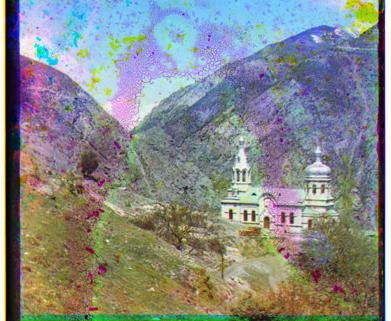
Figure 4. 00056v.jpg - Cathedral using NCC
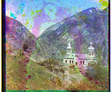
Figure 5. 00056v.jpg - Cathedral using L2
I lost an hour to this. np.roll wraps pixels around, which is fine for building the final image (the wrapped edge gets cropped) but wrong for scoring, because wrapped content from the opposite edge ends up inside the metric.
original   [ A B C D E ]
np.roll +1 [ E A B C D ]   <- E wrapped in from the other side

scoring uses only the true overlap:
reference  [ A B C D ]
moving     [ A B C D ]
So during search I slice the overlapping region of the moving image directly , skipping candidates that leave the image. That gives no wraparound and no full-image copy; np.roll is used exactly once per channel at the end.
Figure 6a. 00056v.jpg - Single-scale L2
Figure 6b. 00056v.jpg - Single-scale NCC
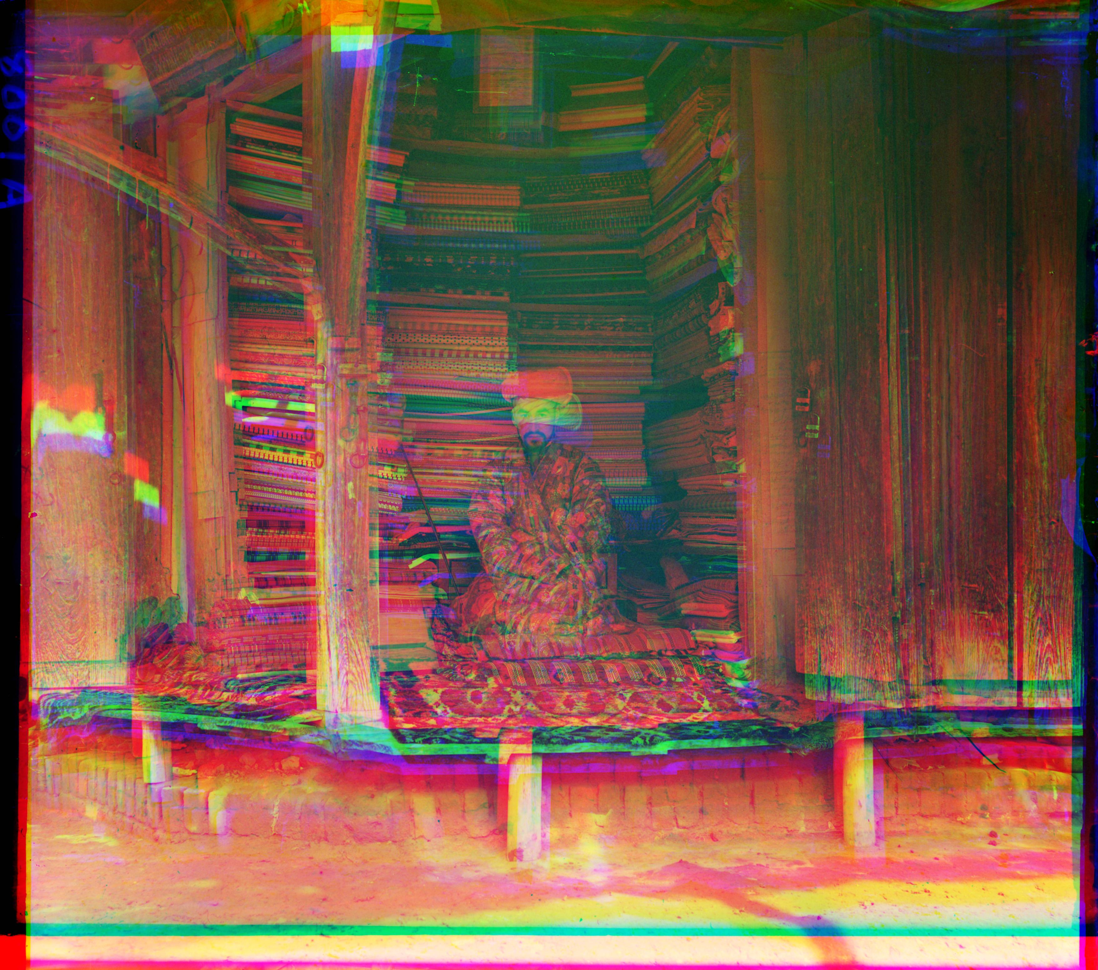
Figure 7a. 01725u.jpg - Single-scale L2
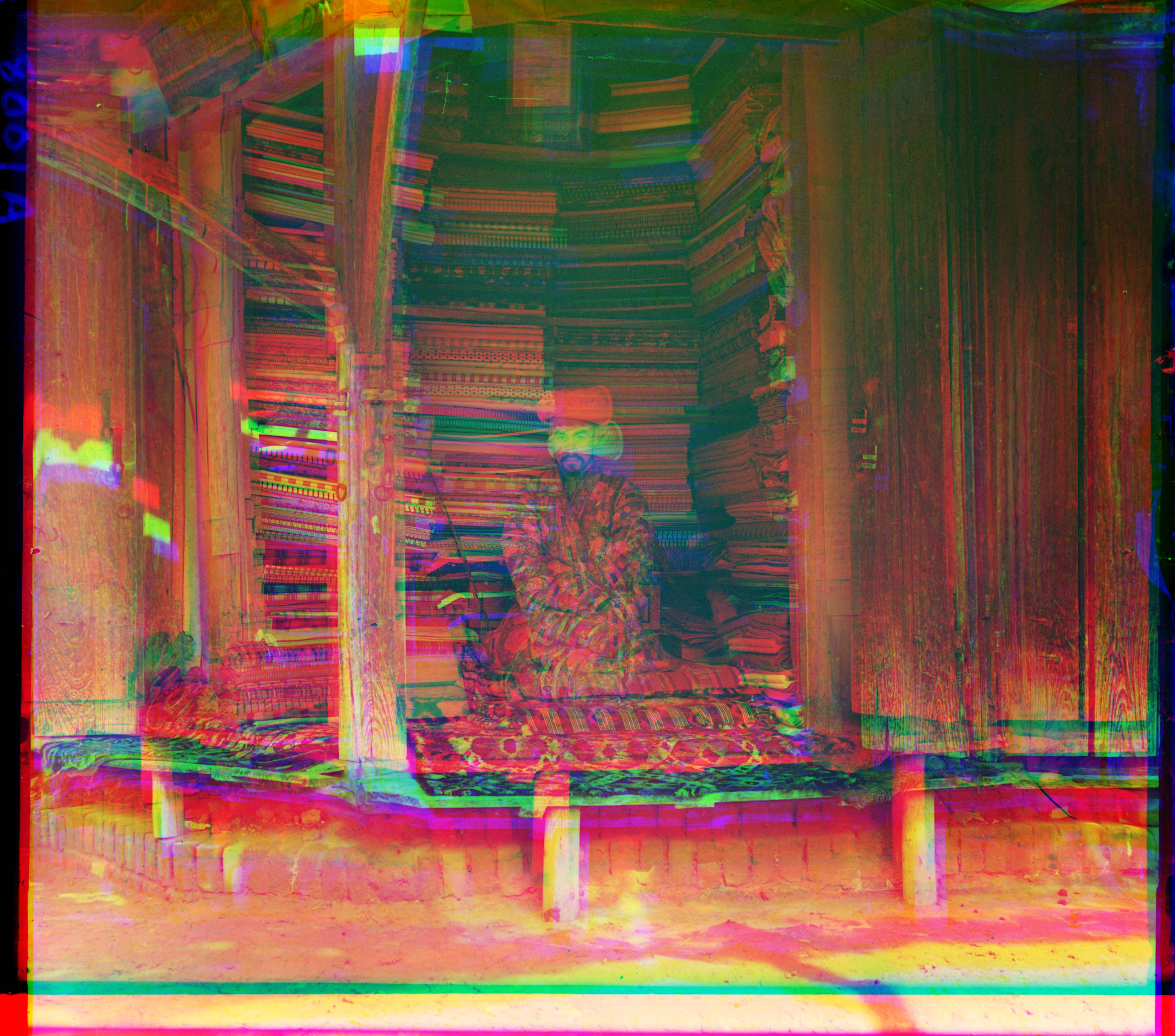
Figure 7b. 01725u.jpg - Single-scale NCC
| IMAGE | Metric | G offset | R offset | Runtime (sec) | Visual result |
|---|---|---|---|---|---|
| 00056v.jpg | L2 | (1, 6) | (1, 13) | 0.41 | Same as NCC |
| NCC | (1, 6) | (1, 13) | 0.45 | Same as L2 | |
| 01725u.jpg | L2 | (15, 15) | (15, 15) | 62.42 | Same as NCC |
| NCC | (15, 15) | (15, -6) | 53.91 | Same as L2 | |
| 00125v.jpg | L2 | (2, 5) | (1, 10) | 0.34 | Same as NCC |
| NCC | (2, 5) | (1, 10) | 0.39 | Same as L2 | |
| 00163v.jpg | L2 | (1, -3) | (1, -4) | 0.35 | Same as NCC |
| NCC | (1, -3) | (1, -4) | 0.35 | Same as L2 | |
| 00458u.jpg | L2 | (9, 15) | (15, 15) | 63.36 | Same as NCC |
| NCC | (9, 15) | (15, 15) | 61.72 | Same as L2 | |
| 00804v.jpg | L2 | (-2, 6) | (-4, 13) | 0.37 | Same as NCC |
| NCC | (-2, 6) | (-4, 13) | 0.34 | Same as L2 | |
| 01007a.jpg | L2 | (13, 15) | (13, 15) | 58.40 | Same as NCC |
| NCC | (13, 15) | (13, 15) | 50.65 | Same as L2 | |
| 01047u.jpg | L2 | (15, 15) | (15, 12) | 53.41 | Same as NCC |
| NCC | (15, 15) | (15, 15) | 69.47 | Same as L2 | |
| 01164v.jpg | L2 | (2, 6) | (3, 11) | 0.37 | Same as NCC |
| NCC | (2, 6) | (3, 11) | 0.35 | Same as L2 | |
| 01269v.jpg | L2 | (2, 6) | (3, 14) | 0.34 | Same as NCC |
| NCC | (2, 6) | (3, 14) | 0.35 | Same as L2 | |
| 01522v.jpg | L2 | (2, 6) | (1, 13) | 0.40 | Same as NCC |
| NCC | (2, 6) | (2, 13) | 0.36 | Same as L2 | |
| 01597v.jpg | L2 | (1, 7) | (1, 15) | 0.36 | Same as NCC |
| NCC | (1, 7) | (1, 15) | 0.36 | Same as L2 | |
| 01598v.jpg | L2 | (0, 8) | (-1, 15) | 0.36 | Same as NCC |
| NCC | (0, 8) | (-1, 15) | 0.34 | Same as L2 | |
| 01657u.jpg | L2 | (7, 15) | (-15, 15) | 54.35 | Same as NCC |
| NCC | (7, 15) | (-15, 15) | 56.22 | Same as L2 | |
| 01728v.jpg | L2 | (1, 8) | (1, 15) | 0.31 | Same as NCC |
| NCC | (1, 8) | (1, 15) | 0.33 | Same as L2 | |
| 01861a.jpg | L2 | (15, 15) | (15, 15) | 51.43 | Same as NCC |
| NCC | (15, 15) | (15, 15) | 47.94 | Same as L2 | |
| 10131v.jpg | L2 | (2, 6) | (3, 12) | 0.33 | Same as NCC |
| NCC | (2, 6) | (3, 12) | 0.34 | Same as L2 | |
| 31421v.jpg | L2 | (0, 8) | (0, 13) | 0.35 | Same as NCC |
| NCC | (0, 8) | (0, 13) | 0.33 | Same as L2 |
On majority (15/18) of the images, NCC and L2 perform similarly. Visually, a human eye can't tell the difference between images processed using different metrics L2 vs NCC. Looking at the results for the second entry in the table (01725u.jpg), we can see that L2 degenerates to the extreme search limit (15, 15) for the Red channel, whereas NCC successfully finds a structurally valid shift of (15, -6). This demonstrates NCC's resilience against boundary brightness artifacts.
On the small 00125v.jpg, single-scale NCC gives G = (2, 5) (score 0.974247) and R = (1, 10) (score 0.947604). Runtime: 0.39 seconds.
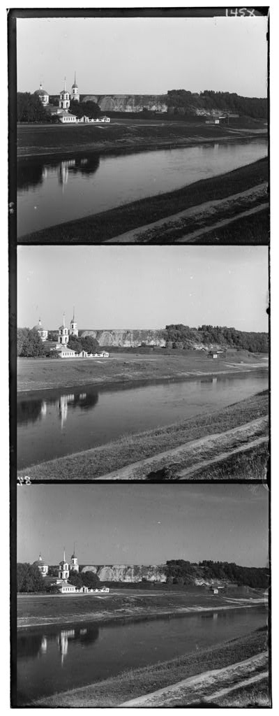
Figure 8a. Original image
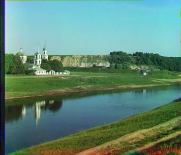
Figure 8b. Single-scale NCC result
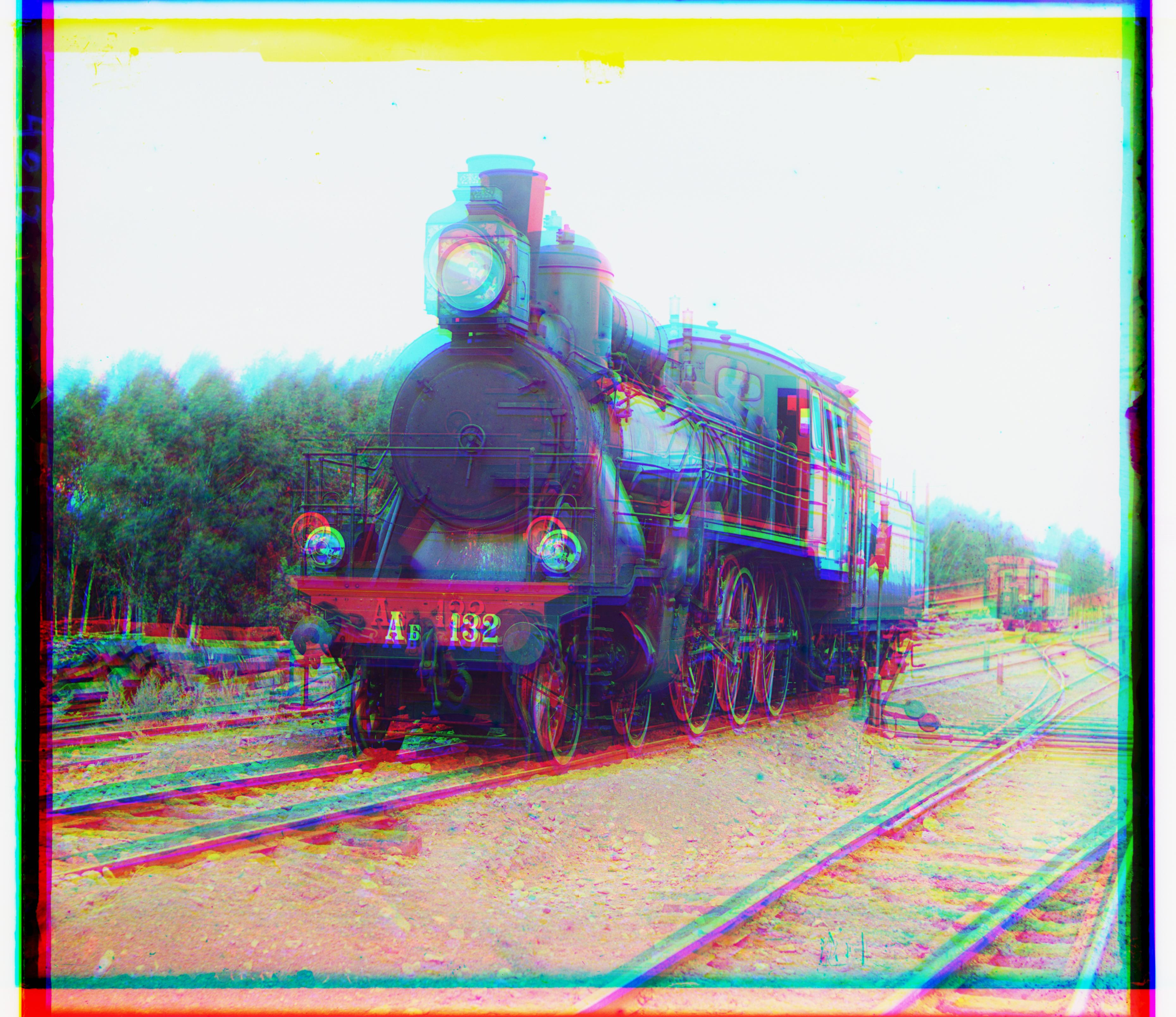
Figure 9a. Radius 15- Runtime 95.41 sec
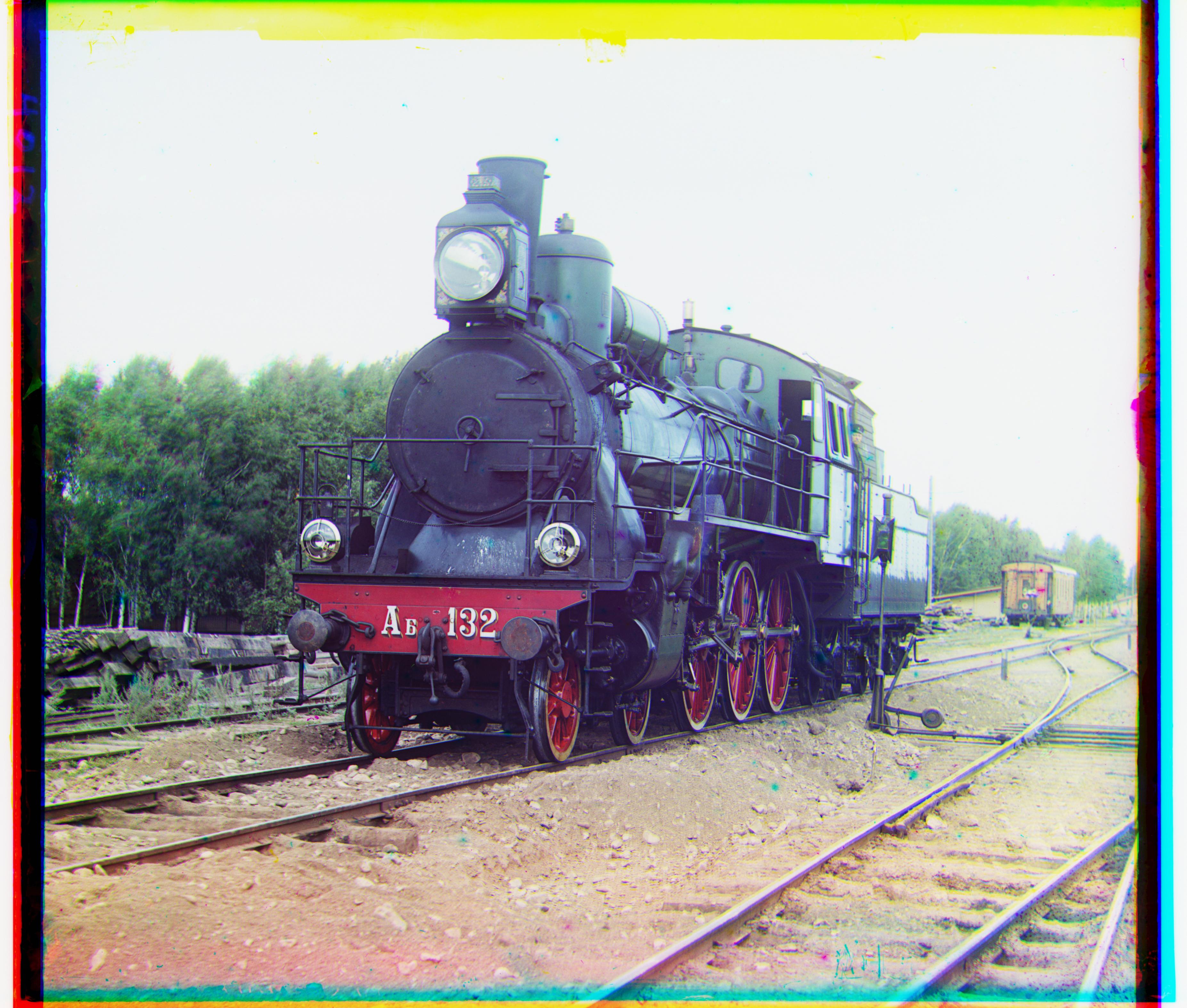
Figure 9b. Radius 130- Runtime 1 hour 53 minutes
Radius 15 is 31×31 = 961 candidates per channel, fine for the small JPEGs. The big TIFFs have displacements of 60-90+ pixels, so covering them means radius ~100, about 201×201 = 40,000 candidates per channel on a much larger image. That is possible to do but doesn't meet the time constraint of sone minute per image the assignment expects.
Before making the image smaller, we apply 5x5 binomial blur with our following filter: [1,4,6,4,1]/16 thanks to Szeliski which is applied vertically and horizontally once. This smooths out small details and keeps the larger structures of image. For instance, when we look at an image which is out of fcous (not very sharp) we miss out the tiny details but the context or a larger edge is still visible.
Not blurring can lead to loss of information in an image which can compromise the image context/details when downsampling an image.
Each level is a 5-tap binomial blur [1,4,6,4,1]/16 followed by taking every other pixel.
After blurring the image, we downsample it to half its height and width. The process is as follows:
Suppose the red channel is shifted by 40 pixels in the original image. At half the resolution, that shift is only about 20 pixels. At quarter resolution, it is only about 10 pixels. So finding the large displacement becomes much easier.
Once we approximate the shift at the coarsest level, we then move up the pyramid level by leve. When moving up, we also double the shift as each level above is double the resolution of the level below it. The pyramid first finds a rough translation on a small image, then uses that translation as a starting point for a smaller search on a larger image.
| Level | Full | 1/2 | 1/4 | 1/8 | 1/16 |
|---|---|---|---|---|---|
| Displacement | 80 px | 40 px | 20 px | 10 px | 5 px |
Instead of searching for an 80 px shift directly, I find a 5 px shift at 1/16, double it going up a level, and search only a small neighborhood around that prediction. Search radii, finest to coarsest, are [5, 5, 5, 7, 15]: the big window is only needed where I'm finding the answer from scratch.
My first version did build the downsampled images, but then the recursion kept passing the full-resolution pair down at every level anyway, so it was really just running five full exhaustive searches back to back, over 200 seconds. I only caught it by printing array.shape at each level and noticing they were all the exact same size.
The basic align_single_scale only ever searched around (0, 0), using range(-r, r+1). But the pyramid needs to search around whatever the coarser level already found, not around zero. So I added center_dx and center_dy, and the search became range(center_dx - r, center_dx + r + 1).
align_single_scale returns (dx, dy, score), but at one point my pyramid code unpacked it as dy, dx, score. Nothing crashed since both are just numbers, so instead of an obvious error I just got a slightly wrong image. I only caught it by checking the printed offsets against what actually moved in the picture.
Going from one pyramid level to the next, the displacement has to be doubled, since each level is half the size of the one below it (center_dx = coarse_dx * 2). I forgot this multiplier at first, and the finer levels ended up searching in completely the wrong spot.
At the smallest pyramid level (1/16 size), the black border around the plate takes up a much bigger chunk of the image than it does at full resolution. That pulled the coarse alignment toward matching the borders instead of the actual photo. Cropping a margin off before scoring the candidates can probably fix it (cropping is partially implemented).
If I set the pyramid too deep, the smallest level could shrink to something like 20×20 pixels while the search radius was still 15, which caused slicing errors. I added a check to stop downsampling once an image gets smaller than about 100 pixels on a side.
Early on I was also calling np.roll() inside the search loop for every single candidate, which means copying a big array over and over. Building the pyramids once up front, slicing directly instead of using np.roll() during search, and using small radii at the finer levels dropped runtime from an incredibly long 200+ seconds runtime to about 14-20 seconds per image, with the same alignment result.
| Image | Single NCC | Runtime Single NCC (sec) | Pyramid NCC | Runtime Pyramid NCC (sec) |
|---|---|---|---|---|
| Train Image | G (10, 15), R (-7, 15) | 81.01 | G (2, 42), R (29, 85) | 16.38 |
On 00458u.jpg the two methods differ in EVERYTHING from G shift to R shift and runtime by a mile! The quality of the images produced by both the methods is therefore different as can be seen by the shift values of G and R in the table above (also below images 10 and 11).
Figure 10. Single-scale
Figure 11. Pyramid
So far, our alignment methods compare the brightness of corresponding pixels. This works when the three exposures have similar brightness, but the glass plate exposures can have very different intensities.
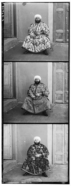
Figure 12. Observe how each exposure on the plate has different brightness
The Emir's robe is a good example. A physical point on the robe may be bright in one exposure but much darker in another. Because raw NCC compares pixel intensities, it can sometimes prefer the wrong alignment that happens to have similar brightness.
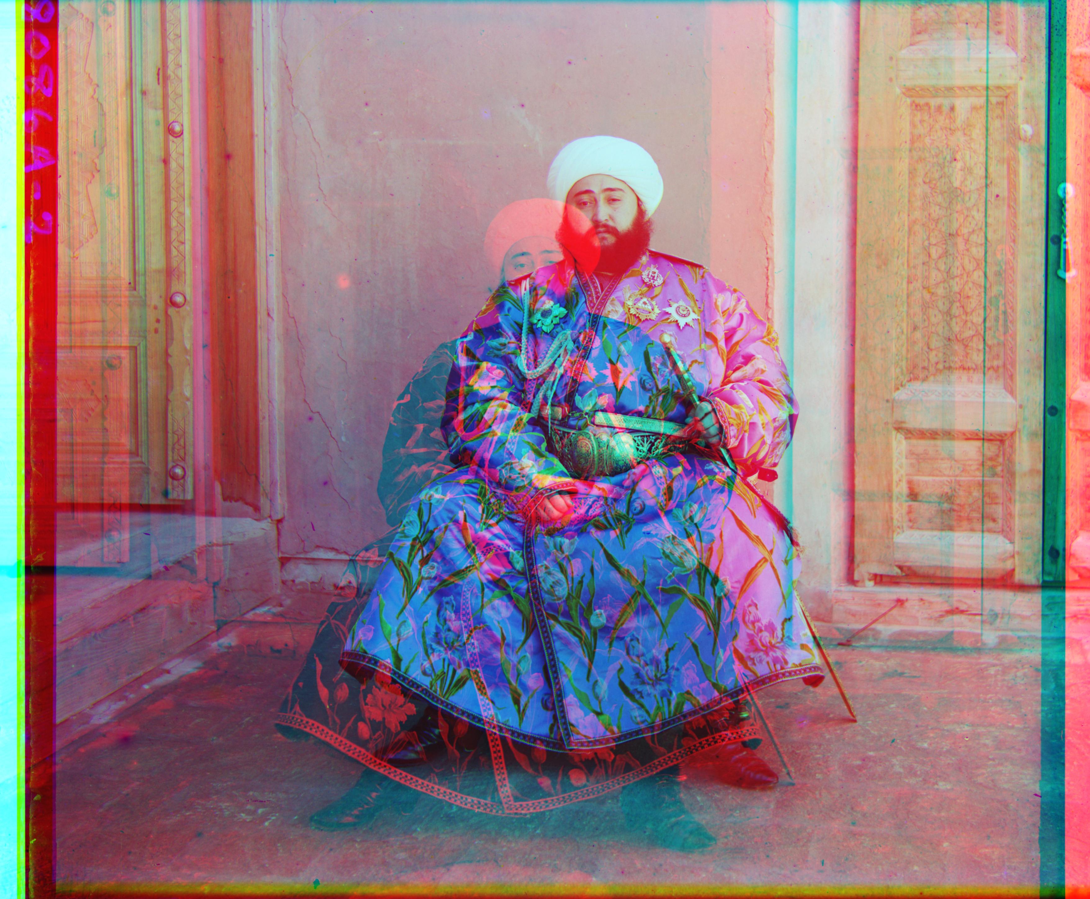
Figure 13a. Raw NCC: wrong. G (24, 49), R (-161, 307)
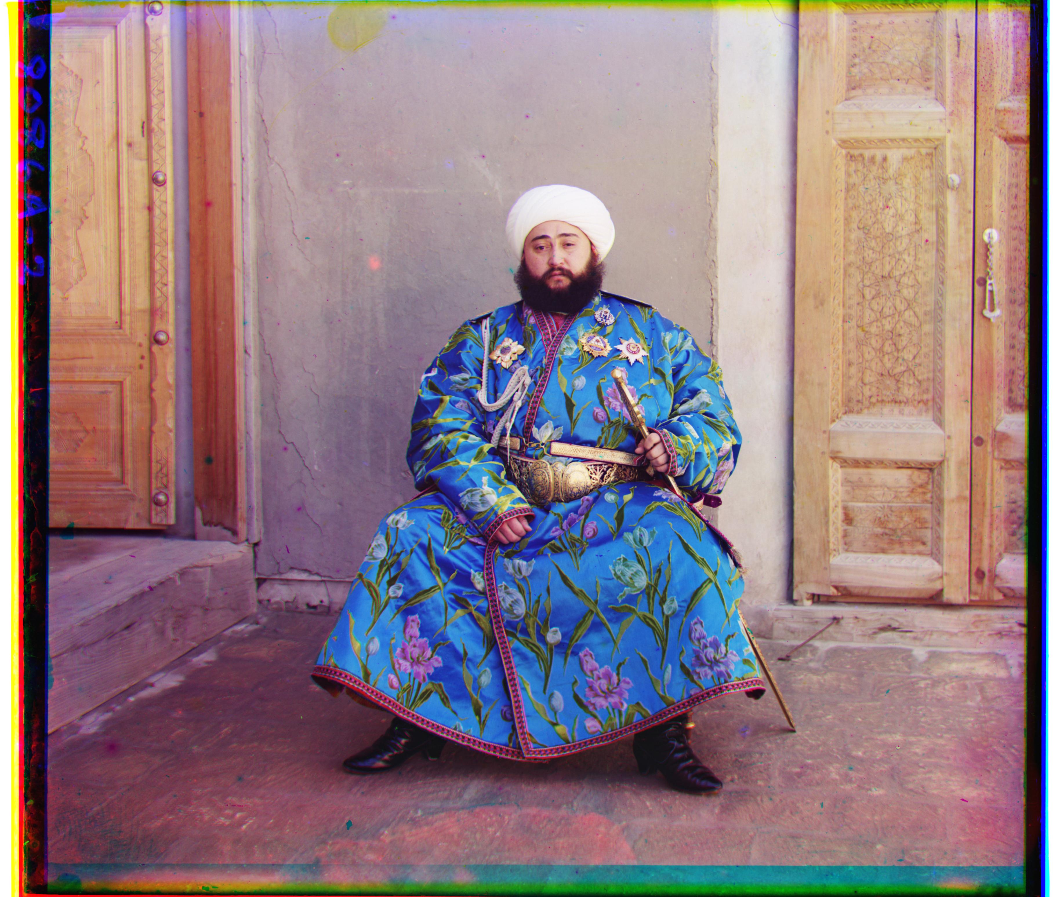
Figure 13b. Gradient NCC: correct. G (24, 49), R (40, 107)
Why gradients over intensity comparison?
Instead of asking "Are these pixels the same brightness?", we ask "Are the edges and structures in the same places?"
We use a Sobel filter to find how quickly the brightness changes around each pixel. Large changes usually occur at edges, such as the boundary of the robe, face, or buildings. We then calculate the gradient magnitude:
gx, gy = Sobel(image) gradient = sqrt(gx*gx + gy*gy)The result is a gradient map that emphasizes edges and other image structure instead of the exact brightness values.

Figure 14. Zoom on the robe using raw NCC.

Figure 15. Zoom on the robe using gradient NCC.
We then run the same NCC alignment process, but on these gradient maps instead of the original intensity images. This makes the alignment less dependent on absolute brightness and more dependent on where the important structures and edges occur.
A reminder that the gradient images are only used to find the shift. Once the shift is found, we apply that shift to the original grayscale channels. The gradients help us decide where to move the image; the original pixels are still used to create the final color image.
After shifting the three color channels into alignment, some pixels near the edges are no longer reliable because the shifted images contain wrapped/invalid border regions. Instead of using a fixed crop for every image, I tried to estimate the valid region automatically.
My approach was to look at the borders of the aligned image and measure how the image (pixels) changes across rows and columns. While doing so, we will look for a strong transition between the artificial border and the actual photgraph. Using this information, I then estimate where might the actual image begin or in other words where is the border starting. Once we figure this out, we then cut off that portion- the border.
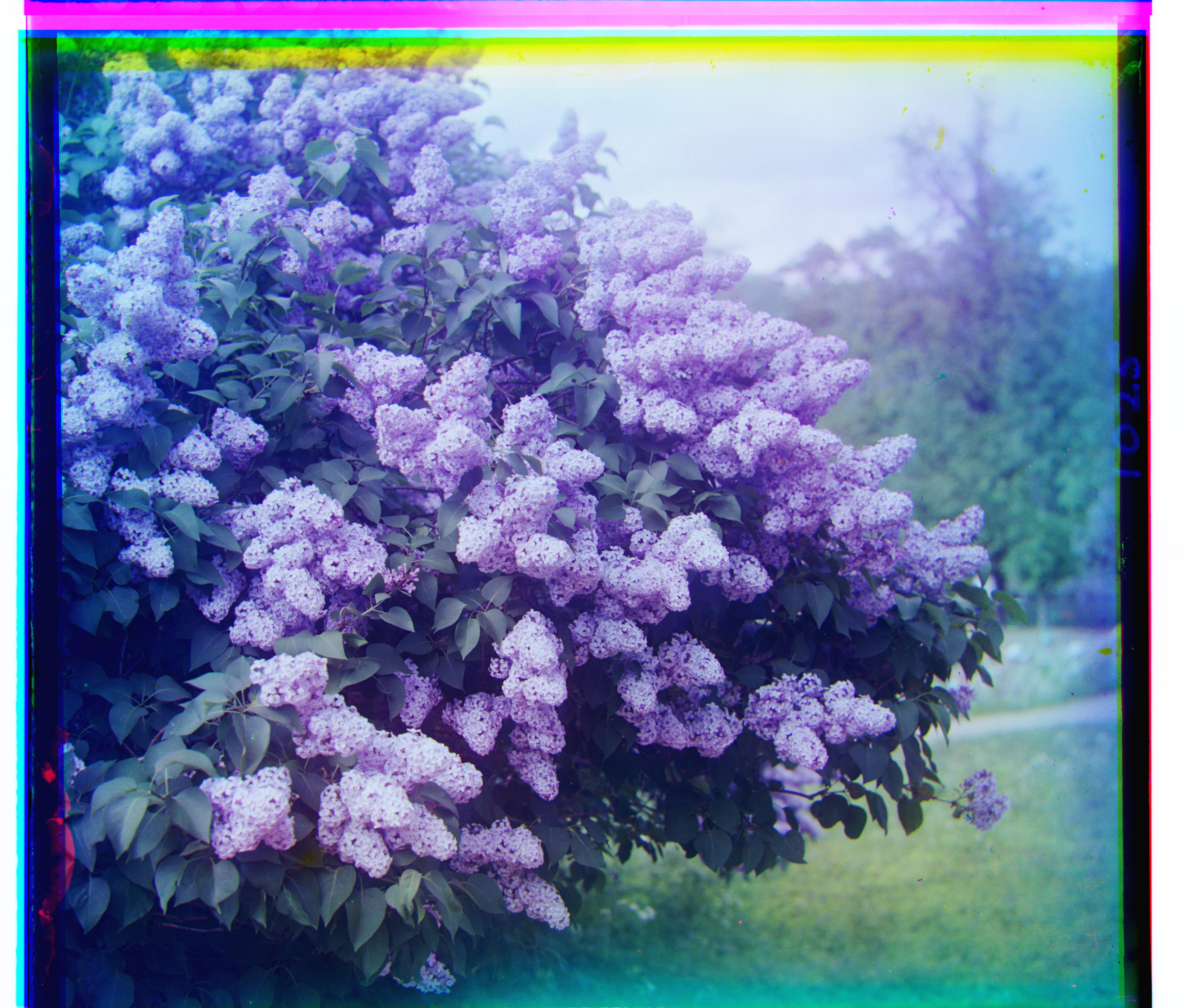
Figure 16. Before crop
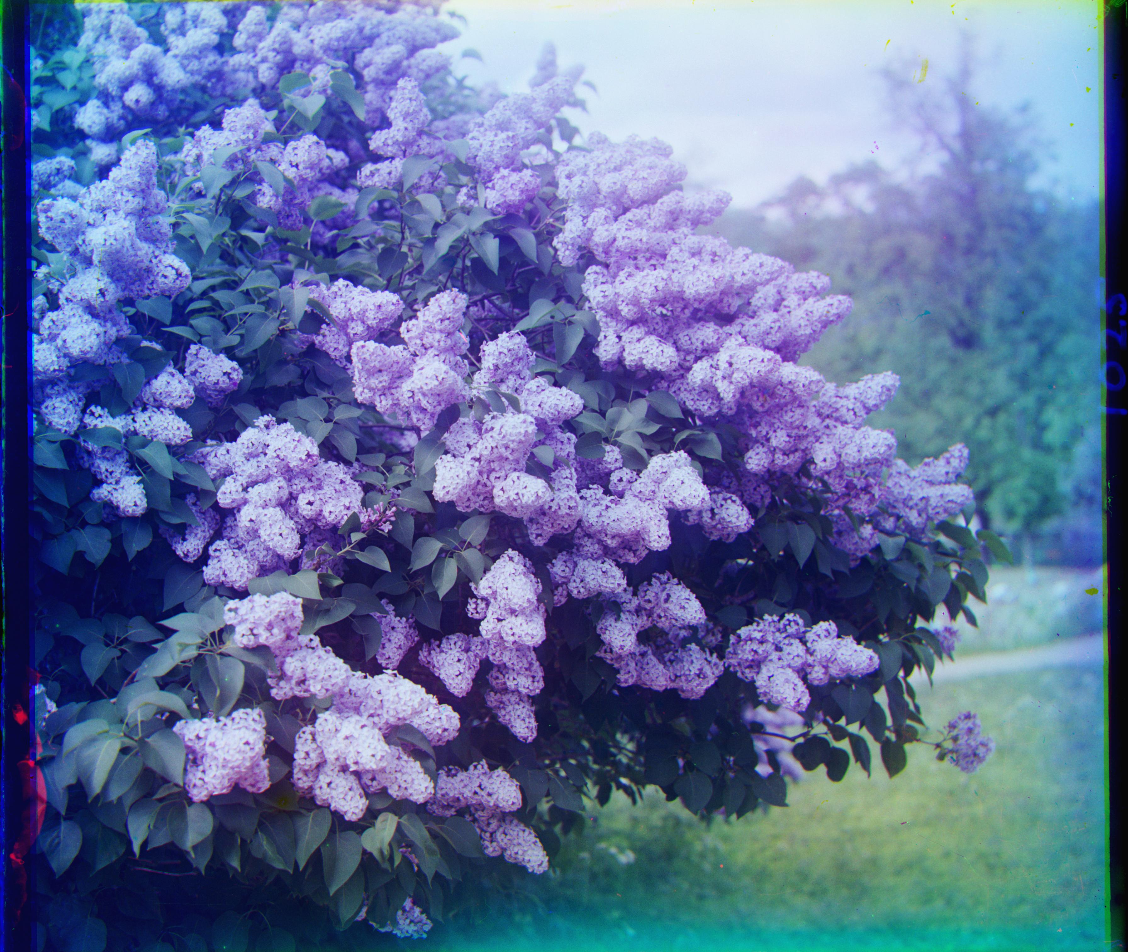
Figure 17. After crop
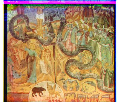
Figure 18. Before crop
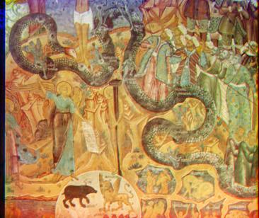
Figure 19. After crop
This worked reasonably well for many images, but it was not perfect. In some photographs (couple of them shown above), strong edges or high-contrast objects near the border looked similar to the artificial boundary.
The algorithm mistake part of the actual photograph for the border and over-crop into the image, removing some valid content. If you focus really closely, you will notice that both the cropped images are losing some part of the actual image from the top
float32 in [0,1]| Parameter | Choice | Why |
|---|---|---|
| Interior margin | 12% | Keeps borders and scan artifacts out of the score |
| Pyramid levels | 5 | An 80 px shift becomes 5 px at 1/16th of the original resolution |
| Radii (fine to coarse) | [5, 5, 5, 7, 15] | Large window only where the answer is found from scratch |
| Single-scale radius | 15 | Enough for the small JPEGs |
| Metric | NCC (L2 also implemented) | Less sensitive to brightness differences between filters |
| Gradient features | Sobel gradient magnitude | Replaces raw pixel values with edge maps. Prevents alignment failure on inter-channel contrast inversions (shown previously in Figures 12 and 13) by focusing purely on shared structural boundaries. |
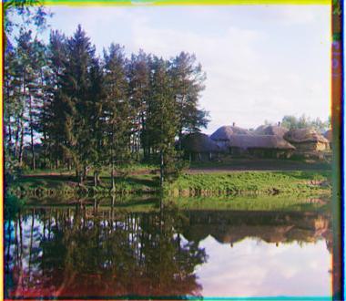
00163v: G (1, -3), R (1, -4)
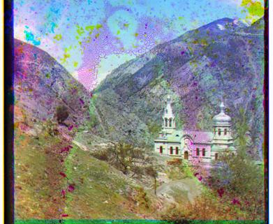
cathedral: G (1, 6), R (1, 13)
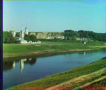
00125v: G (2, 5), R (1, 10)
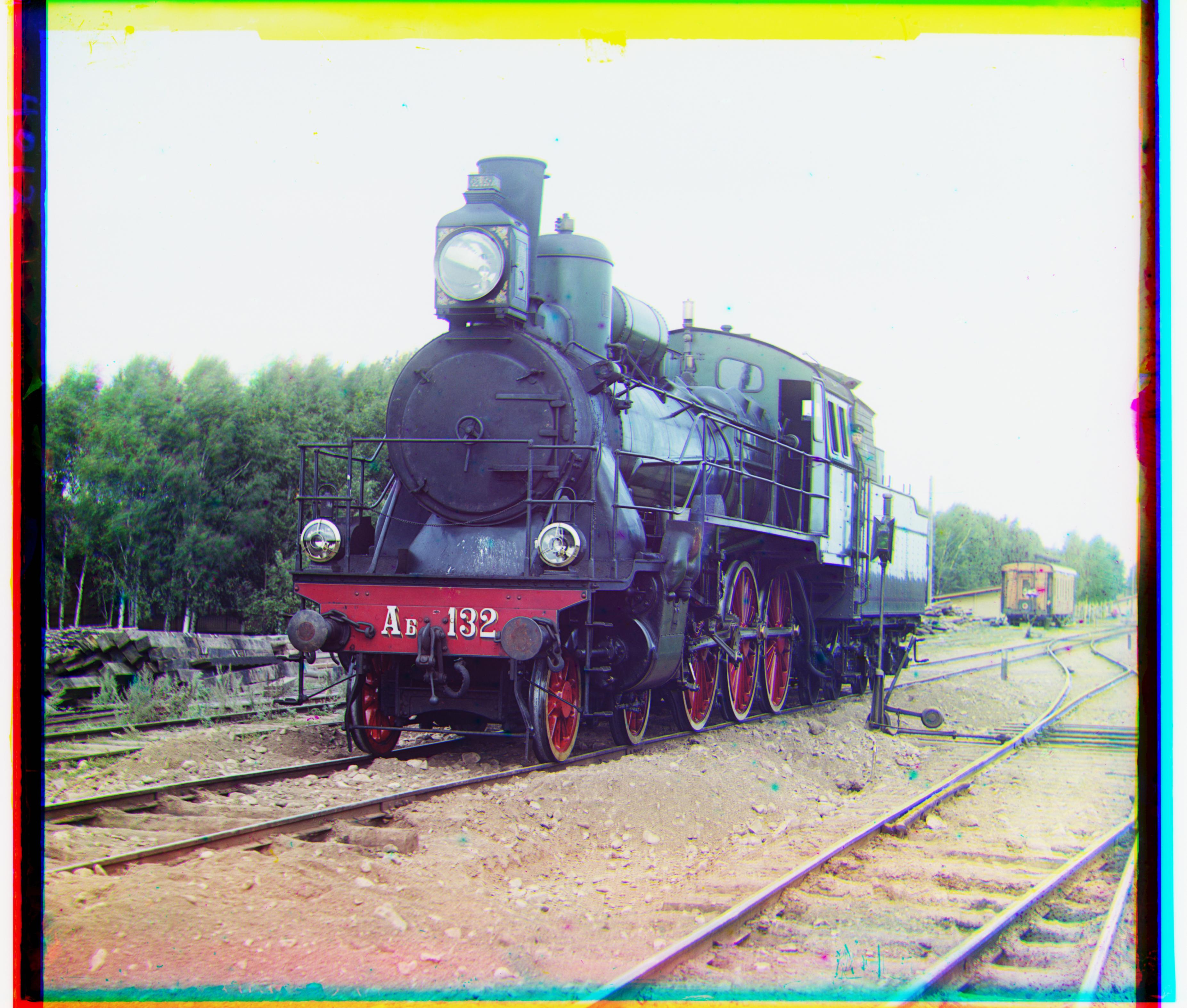
00458u: G (2, 42), R (29, 85)
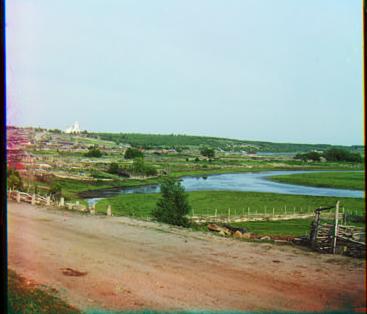
00804v: G (-2, 6), R (-4, 13)
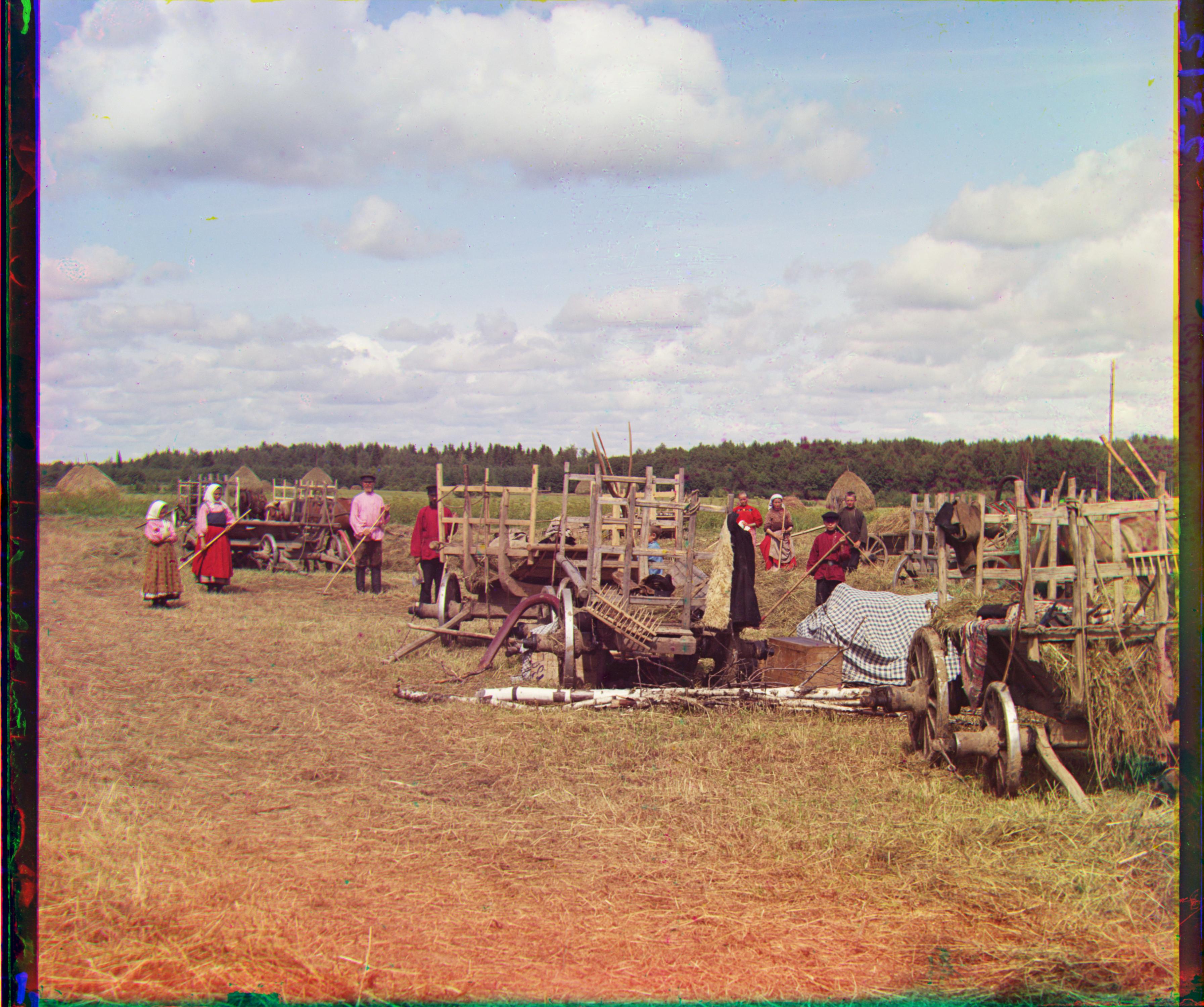
01007a: G (14, 60), R (13, 129)
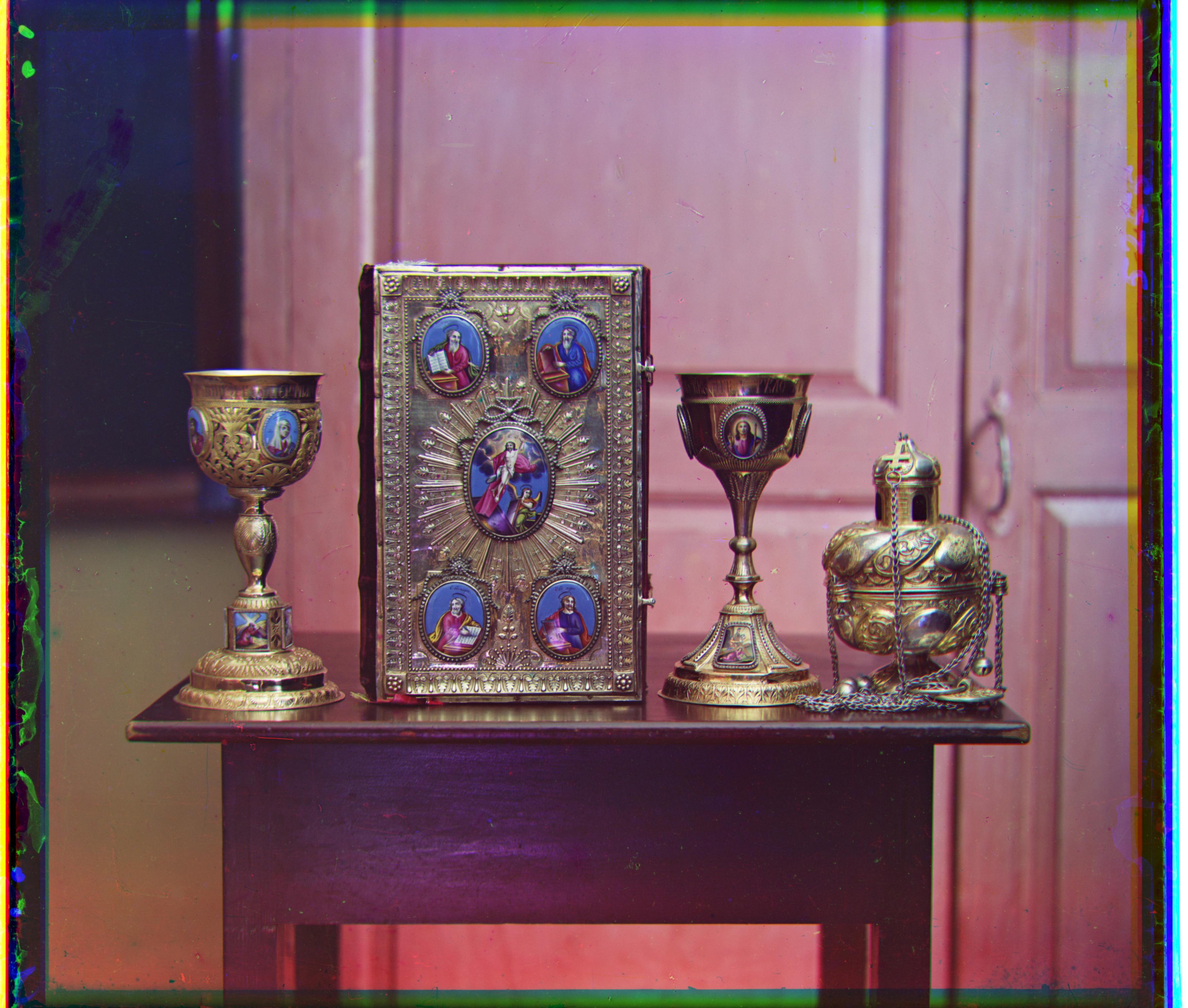
01047u: G (20, 25), R (33, 71)
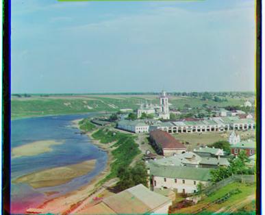
01164v: G (2, 6), R (3, 11)
01269v: G (2, 6), R (3, 13)
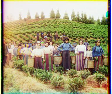
01522v: G (2, 6), R (2, 13)
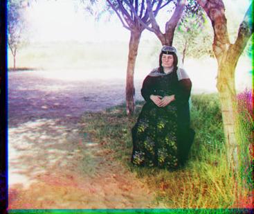
01597v: G (1, 7), R (1, 16)
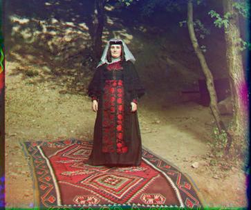
01598v: G (0, 8), R (-1, 17)
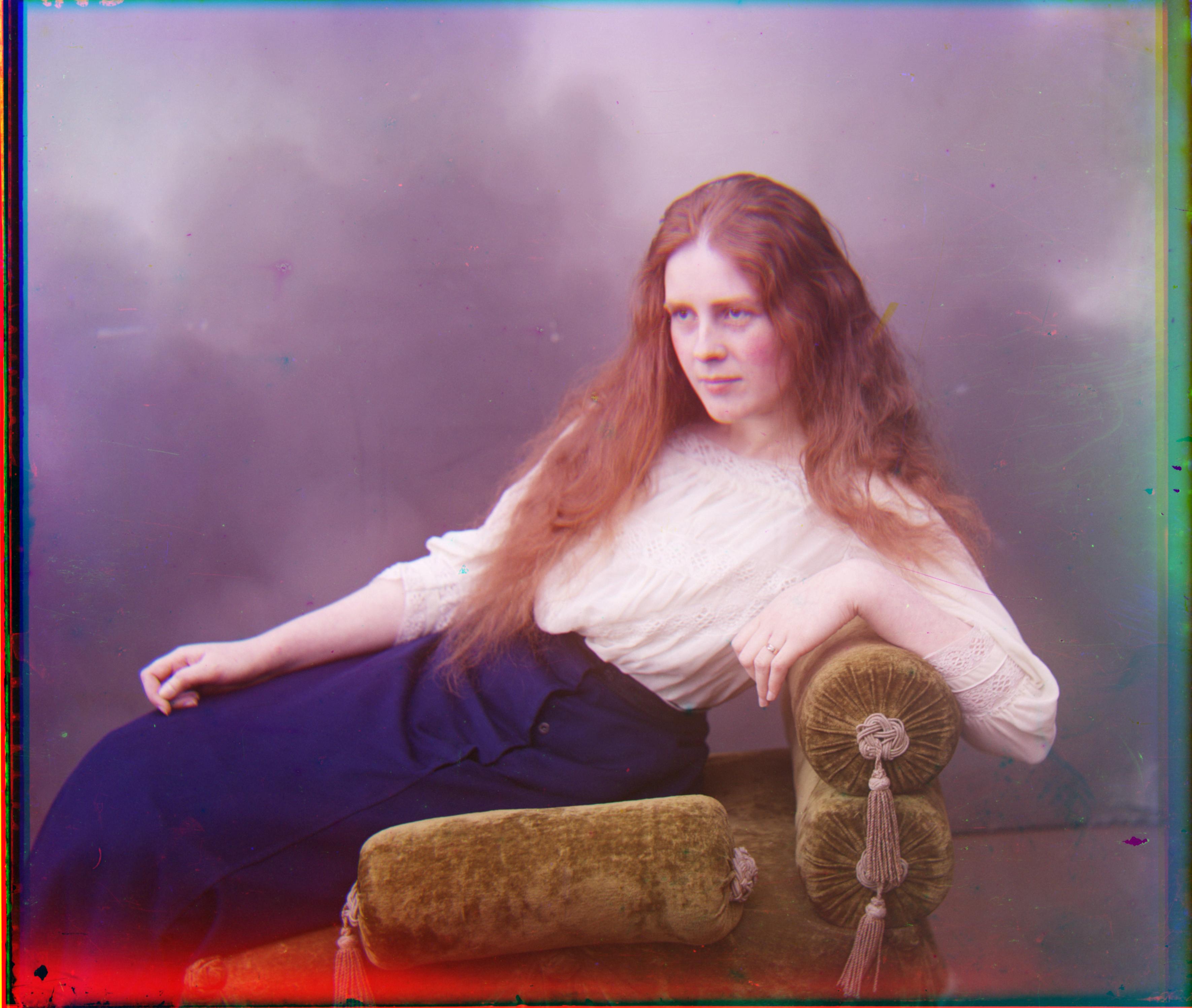
01657u: G (9, 56), R (13, 120)
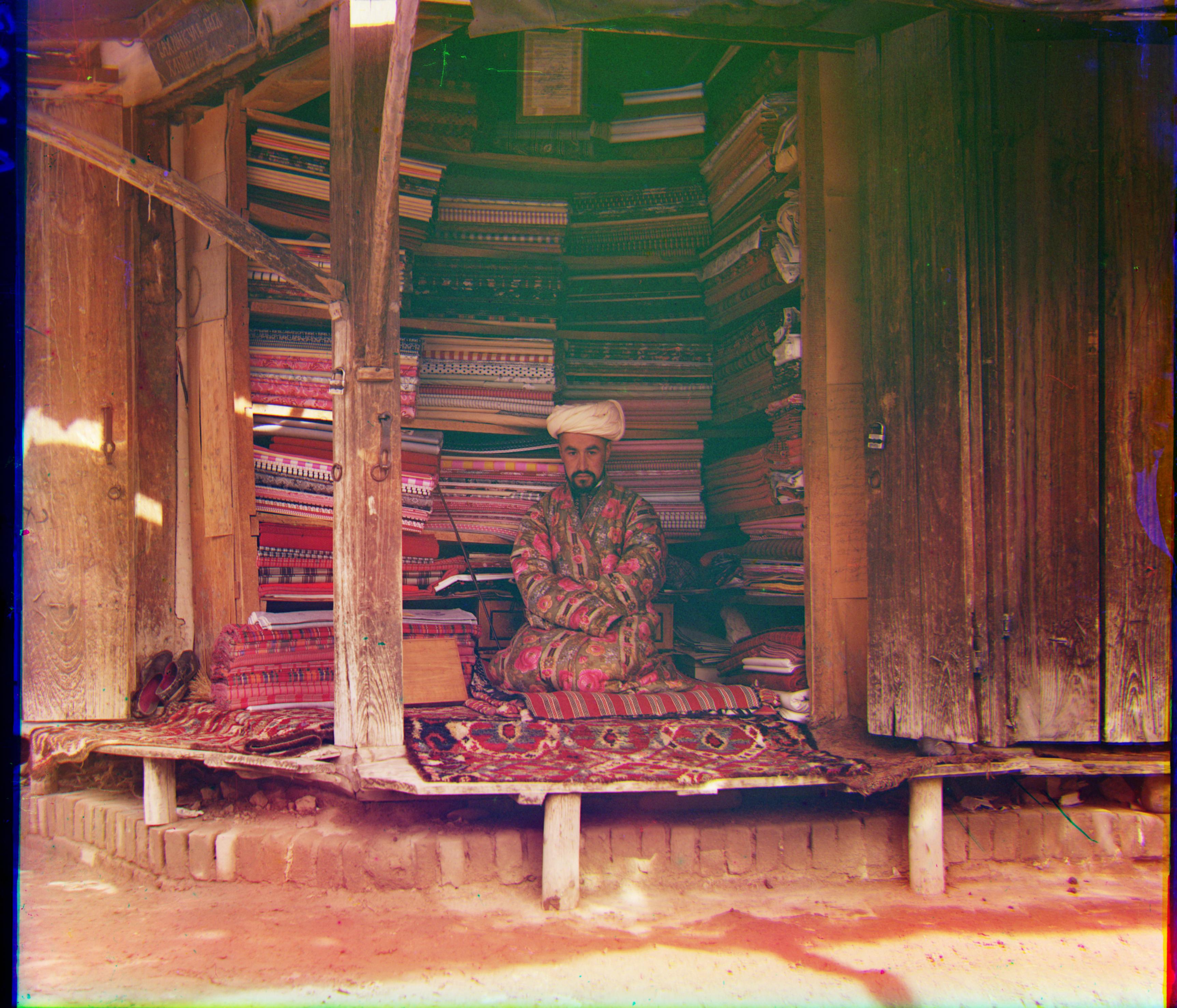
01725u: G (44, 76), R (77, 162)
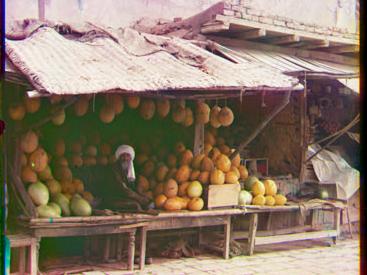
01728v: G (1, 8), R (1, 18)
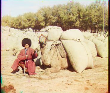
01861a: G (39, 71), R (62, 147)
10131v: G (2, 6), R (3, 12)
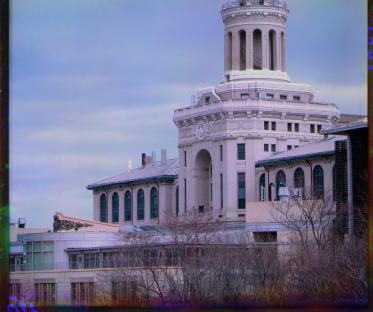
31421v: G (0, 8), R (0, 13)
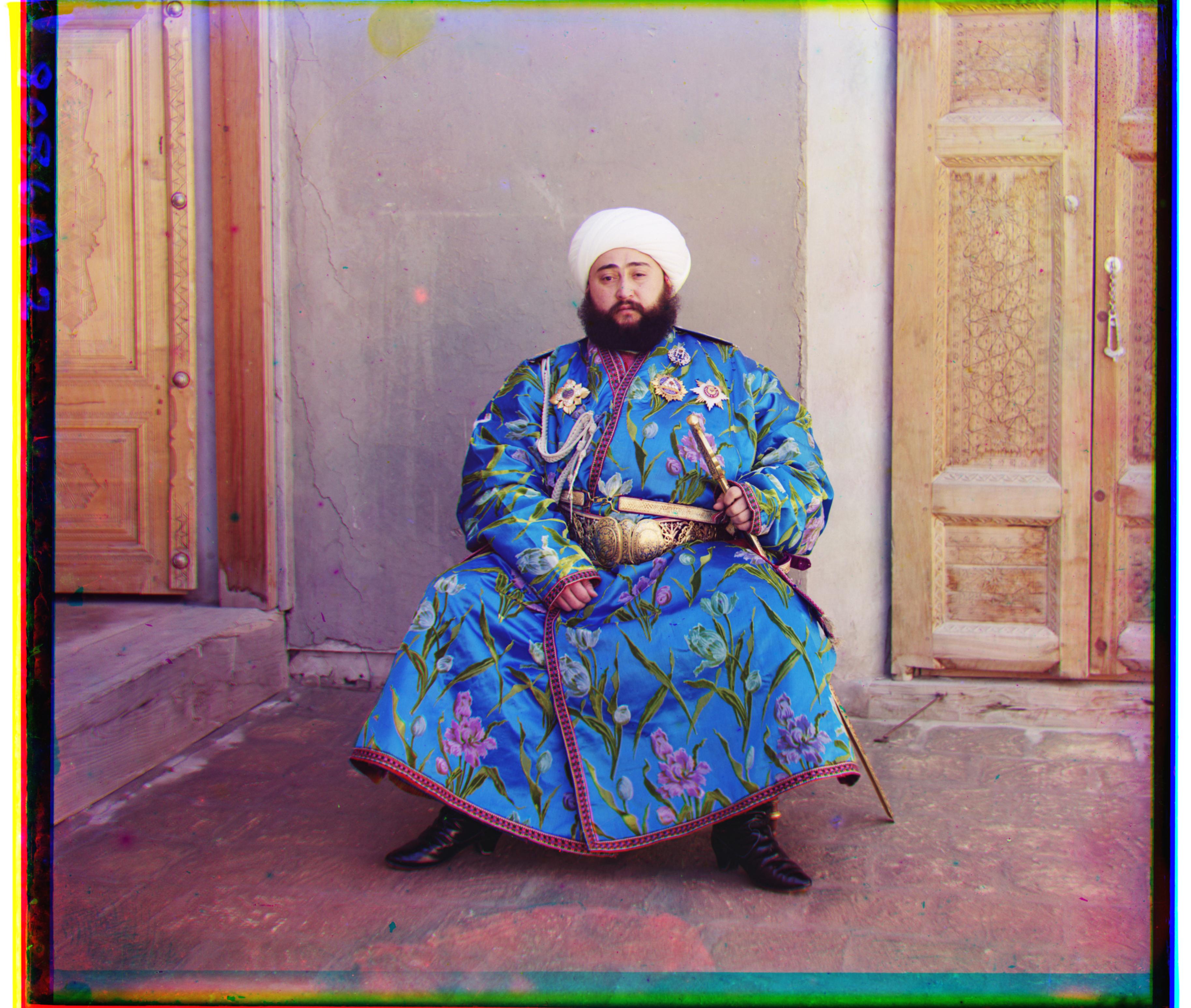
Ėmir Bukharskīĭ Bukhara: G (24, 49), R (40, 107)
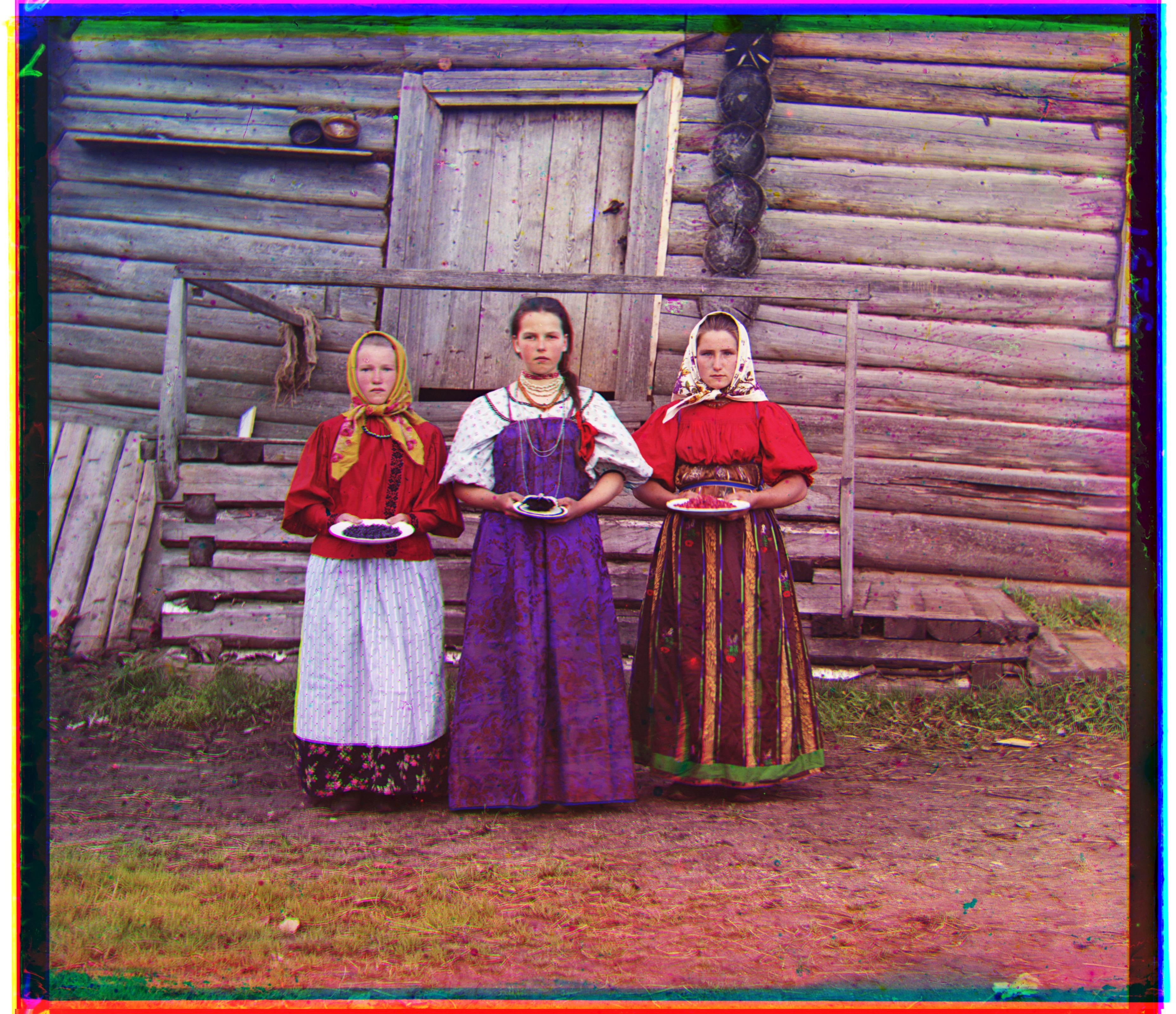
3 Ladies: G (9, -14), R (15, 12)
Flower: G (-6, 49), R (-24, 96)
The automatic border detector is surprisingly tricky. Cropping seemed to work on majority of the images however for a few images (among which some are Figure 16, 17, 18 and 19) the cropping heristic seemed to over-crop the images; specifically from the top.
np.roll wraparoundnp.roll wraparound was another issue. It is convenient for applying the final alignment shifts, but it wraps pixels around the image edges. Those wrapped regions are not valid, so they need to be removed before constructing the final RGB image.
One of the most obvious bugs I encountered was misaligning the color channels which I placed in the wrong order when I reconstructed the final image.
As I was splitting the image in the order B, G, R, I trivially thought that same sequence would apply to the final image processing. I was doing the following:
color_image = np.stack([B_cropped, G_cropped, R_cropped],axis=2)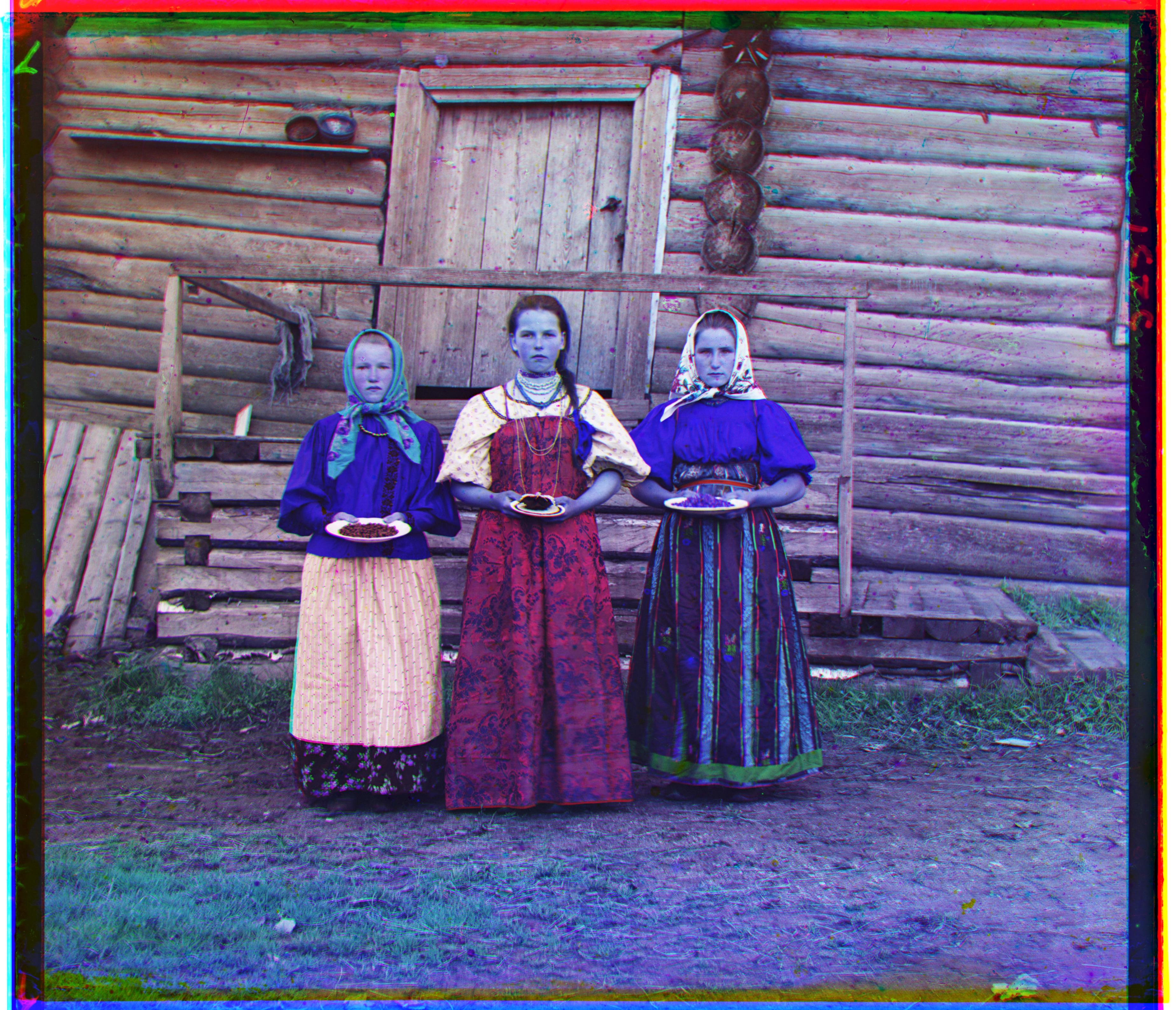
Figure 20. Blue tint
Figure 21. Fixed color sequence
It was until I saw that the faces were blue and that clicked instantly that it might be a reconstruction issue since the images, eventhough had a blue tint, were coming out sharp. So I simply swapped the order of the channels as follows:
color_image = np.stack([R_cropped, G_cropped, B_cropped],axis=2)
This assignment looked like "shift three images until they line up". Most of the work was making stages agree with each other: dtype, what (dx, dy) means at every call site, how a displacement at a coarse pyramid level scales back to full resolution, and the difference between the feature I align on and the pixels I output. It was less about knowing the formula and more about making sure every stage of the pipeline agrees on what a coordinate means.
Coarse-to-fine search is much more than just a speed trick. The image pyramid changes a large alignment problem into a sequence of smaller ones. A rough displacement can be found at low resolution and then refined as the image gets larger. This made it possible to align high-resolution plates without exhaustively searching a huge range of full-resolution shifts- it reduced the runtime by 10-15 times!!!
When pixels are unreliable, features can be better.
Processing .tif files showed that raw intensity is not always the best thing to align. Using gradient magnitude emphasized edges and structure instead of absolute brightness, which gave the algorithm another way to recognize corresponding features. It was so satisfying to understand what it was doing. Instead of camparing the pixel to pixel intensities, it compares the rate of change in intensity (gradient) which is more robust to brightness differences between channels.
Small implementation mistakes can create surprisingly convincing errors.
Swapping dx and dy, reversing the channel order, or mishandling the coordinate scaling in the pyramid can still produce an image that looks almost reasonable. The blue-face bug was a good reminder that even if the alignment itself is correct, the final RGB reconstruction can still be wrong.
Alignment and reconstruction are two different problems. I can use cropped regions or gradient images to decide where two channels line up, but I still need to apply those shifts to the original channels to preserve the actual image. Separating the data used for alignment from the data used for output made the pipeline much easier to reason about.
Automatic processing is not automatically reliable. The automatic cropping experiment showed this especially clearly. A rule that works well on one photograph can fail on another because real image content can look like a border. In some cases, the detector over-cropped into the photograph. This made me more aware that computer vision algorithms need to be evaluated on different images rather than judged from one successful example.
Visual debugging is extremely valuable and what better opportunity to do it then Computer "Vision"? Looking only at the numerical offsets or similarity scores would have made several problems difficult to notice. Comparing the actual images immediately revealed issues such as color-channel swaps, misalignment, wrapped borders, and over-cropping.
For image-processing problems, the output image itself is often one of the best debugging tools.